|
|
 |
|
|
|
|
| |
|
|
|
Lower Atmosphere
Read more |
Distribution & concentration (1)
We learned a lot about the gases in our atmosphere, in particular in the troposphere, the lowest layer of the atmosphere. Here we find countless chemical compounds. But concentrations and distributions are strongly varying.
|
|
|
|
|
|
How to decribe a gas in the atmosphere?
Amount
A gas in the atmosphere can be:
a) a major component of the air (oxygen, nitrogen, argon)
b) a major trace gas (carbon dioxide, methane, ozone, nitrogen dioxide, ...)
c) a minor trace gas (many organic gases as butane, ethanol, but also CFCs, ...)
Trace gases are gases which make up only for a tiny fraction of the air, this can be less than one molecule among one billion or even one trillion of air molecules.
|
|
|
Can you imagine one ppb?
ppb = parts per billion (American *)
more corrcet: nmol/mol
1 molecule among 1,000,000,000
1 Indian in all India, 1 cent in 10 Mio EURO, 1 second in 32 years.
And 1 ppt?
ppt = parts per trillion
more correct: pmol/mol
1 molecule among
1,000,000,000,000
1 stamp in the area size of Paris ...
It is so little, beyond our imagination, but modern science can detect it.
| | |
*The misunderstanding of mixing ratio 'units' ppm and ppb
In numerous scientific publication the amount of a compound in the air is given in ppm (parts per million) or ppb (parts per billion). We also use this abbreviation here, because it is so common and you find it everywhere. But they are very misleading.
Three typical mistakes:
1) Often it is written: The concentration of CO2 in the air is 370 ppm. This is wrong. 370 ppm is a mixing ratio and not a concentration. Concentrations are for example mass per volume like the ozone concentration 100 µg / m3. They have a real unit.
2) Mixing ratios do not really have a unit. Because you can cancel the units. They describe only that you have 370 molecules among 1,000,000 molecules, if you have 370 ppm. The more correct expression is: 370 µmol/mol.
3) The term billion and trillion is defined in different ways in different countries:
1 American billion = 1 British milliard (seldom used) = 1,000,000,000
1 American trillion = 1 British billion (seldom used) = 1,000,000,000,000
In many other languages (French: milliard, German: Milliarde) terms related to 1 British milliard are more common than the American billion for 109. So, do not mix it up!
|
often used: |
more correct: |
it means: |
|
ppm (parts per million) |
µmol / mol = 10-6
(micromol / mol) |
1 of 1,000,000 |
|
ppb (parts per billion) American |
nmol / mol = 10-9
(nanomol / mol) |
1 of 1,000,000,000 |
|
ppt (parts per trillion) American |
pmol / mol = 10-12
(pikomol / mol) |
1 of 1,000,000,000,000 |
|
Distribution
Depending on local and temporary conditions, a gas in the atmosphere can be:
|
 |
|
|
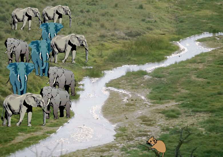
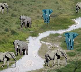
1. a) homogeneously distributed
(e.g. nitrogen, oxygen, carbon dioxide)
image: Elmar Uherek
|
|
|
 |
|
|
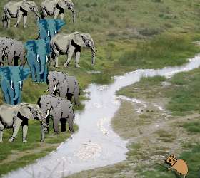
b) inhomogeneously distributed
(e.g. water vapour, ozone, many minor trace gases)
|
|
|
Homogeneously means, that we find comparable mixing ratios of the gas everywhere around the globe and also for varying altitudes. This is the case for stable gases with a long life time. They are only slowly removed from the atmosphere and do not react or only in minor amounts.
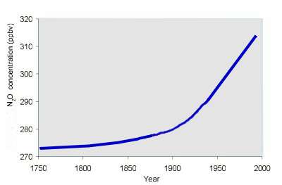
Example: Nitrous oxide N2O |
 |
|
|
2. Distribution of nitrous oxide in the atmosphere. Measured over the pacific ocean in different altitudes and latitudes. Error bars are shown.
J.E. Collins et al., J. of Geophys. Research, 101, D1 (1996) p. 1975-84
|
Nitrous oxide N2O is an homogeneously distributed gas. However, the concentration has been increasing during the recent 200 years mainly due to human activity.
3. Graph: Elmar Uherek
|
|
|
 |
|
|
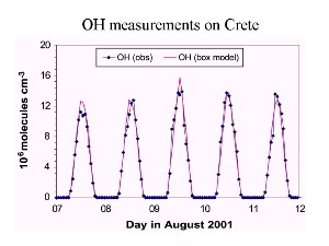
4. Time profile of OH concentrations.
Source: Presentation J. Lelieveld MPI Mainz 2003
|
|
|
Development in time
The abundance of gases can strongly depend on the sun, if they are involved in chemical processes, where photolysis plays a role. In this case they have a daily pattern and sometimes also a seasonal pattern.
Daily variation: example hydroxyl radical OH
OH, for example depends on the sunlight, rises during daytime and decreases at night, es decribed in the unit oxidation.
|
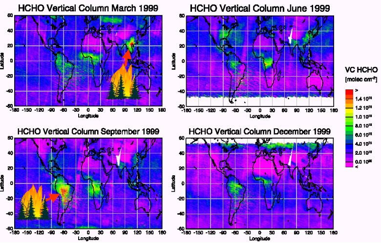
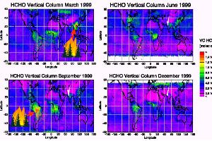
Seasonal variation: example formaldehyde
Formaldehyde HCHO is a gas which is for example produced during vegetation fires. Observed from the satellite based GOME instrument it can be seen that concentrations are high during the fires seasons (March in Southeast-Asia, September in Brazil).
|
|
 |
|
|
5. Formaldehyde - total columns observed by GOME from space.
© IUP Bremen / ESA - GOME
Please click to enlarge (110 K)
|
|
|
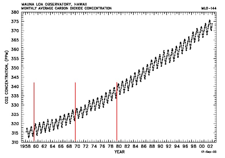
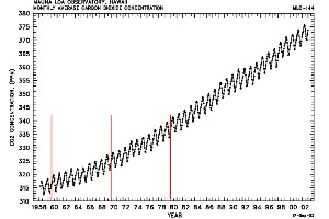
Some gases increase or decrease in the long term over decades, hundreds, thousands or even millions of years. Human activity caused an average increase of many gases during the last 200 years after beginning industrialisation as already shown for N2O.
|
 |
|
|
6. Trend in CO2 concentrations recorded at the Mauna Loa Observatory, Hawaii
graph: © CDIAC US Department of Energy
Please click for full view! (70 K)
|
|
|
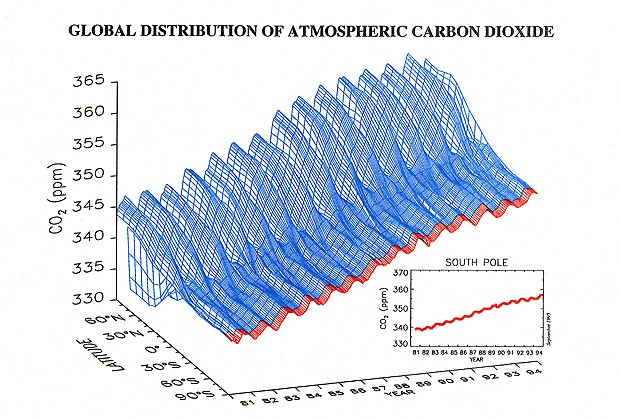
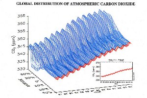
Growing season and human impact: example carbon dioxide (CO2)
Carbon dioxide is an excellent example to study the global distribution of a gas. It is rather stable and therefore distributes over the whole globe. But we know: Due to human activity carbon dioxide is continuously increasing over the years, as shown on the left.
Most of the CO2 is formed on the northern hemisphere because here is the bigger land mass and much more people are living here and are consuming energy (think about Europe, the US, China and India).
|
 |
|
|
7. Global CO2 distribution and annual and mid-term variation
© NOAA / CMDL
Please click to enlarge! (90 K)
|
|
|
Therefore carbon dioxide increases first in the northern hemisphere and after that slowly finds its way to the south. The transport over the equator takes time, since mixing within one hemisphere is faster than mixing between the hemispheres.
But we observe something else: The annual pattern of CO2 varies. In winter trees and other plants stop growing. They take up less CO2. At the same time humans begin to heat their houses and emit more CO2. Consequently we have the highest concentrations at the end of the heating period in May and about 5 ppm less CO2 after the end of the growing period in October. The two graphs clearly show both patterns.
|
About this page:
author: Dr. Elmar Uherek - Max Planck Institute for Chemistry, Mainz
scientific reviewer: Dr. Rolf Sander - Max Planck Institute for Chemistry, Mainz - 2004-05-18
last published: 2004-05-24
|
|
|
|